Visualizing the Lotka-Volterra Model
The Lotka-Volterra equations are a set of coupled ordinary differential equations(ODEs) that can be used to model predator prey relationships.
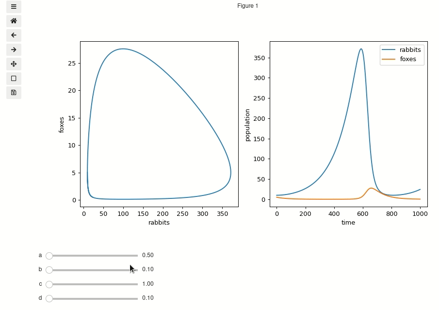
They have 4 parameters that can each be tuned individually which will affect how the flucuations in population behave. In order to explore this 4D parameter space we can use mpl_interactions’ plot function to plot the results of the integrated ODE and have the plot update automatically as we update the parameters.
Define the function
[ ]:
%matplotlib ipympl
import matplotlib.pyplot as plt
import numpy as np

from mpl_interactions import ipyplot as iplt
[ ]:
# this cell is based on https://scipy-cookbook.readthedocs.io/items/LoktaVolterraTutorial.html
from scipy import integrate

t = np.linspace(0, 15, 1000)  # time
X0 = np.array([10, 5])  # initials conditions: 10 rabbits and 5 foxes


def f(a, b, c, d):
    def dX_dt(X, t=0):
        """ Return the growth rate of fox and rabbit populations. """
        rabbits, foxes = X
        dRabbit_dt = a * rabbits - b * foxes * rabbits
        dFox_dt = -c * foxes + d * b * rabbits * foxes
        return [dRabbit_dt, dFox_dt]

    X, _ = integrate.odeint(dX_dt, X0, t, full_output=True)
    return X  # expects shape (N, 2)
Make the plots
Here we make two plots. On the left is a parametric plot that shows all the possible combinations of rabbits and foxes that we can have. The plot on the right has time on the X axis and shows how the fox and rabbit populations evolve in time.
[ ]:
fig, (ax1, ax2) = plt.subplots(ncols=2, figsize=(10, 4.8))
controls = iplt.plot(
    f, ax=ax1, a=(0.5, 2), b=(0.1, 3), c=(1, 3), d=(0.1, 2), parametric=True
)
ax1.set_xlabel("rabbits")
ax1.set_ylabel("foxes")

iplt.plot(f, ax=ax2, controls=controls, label=["rabbits", "foxes"])
ax2.set_xlabel("time")
ax2.set_ylabel("population")
_ = ax2.legend()
You may have noticed that it looks as though we will end up calling our function f twice every time we update the parameters. This would be a bummer because then our computer would be doing twice as much work as it needs to. Forutunately the control object implements a cache and will avoid call a function more than necessary when we move the sliders.
If for some reason you want to disable this you can disable it by setting the use_cache attribute to False:
controls.use_cache = False
[ ]: