Hyperslicer Tutorial#
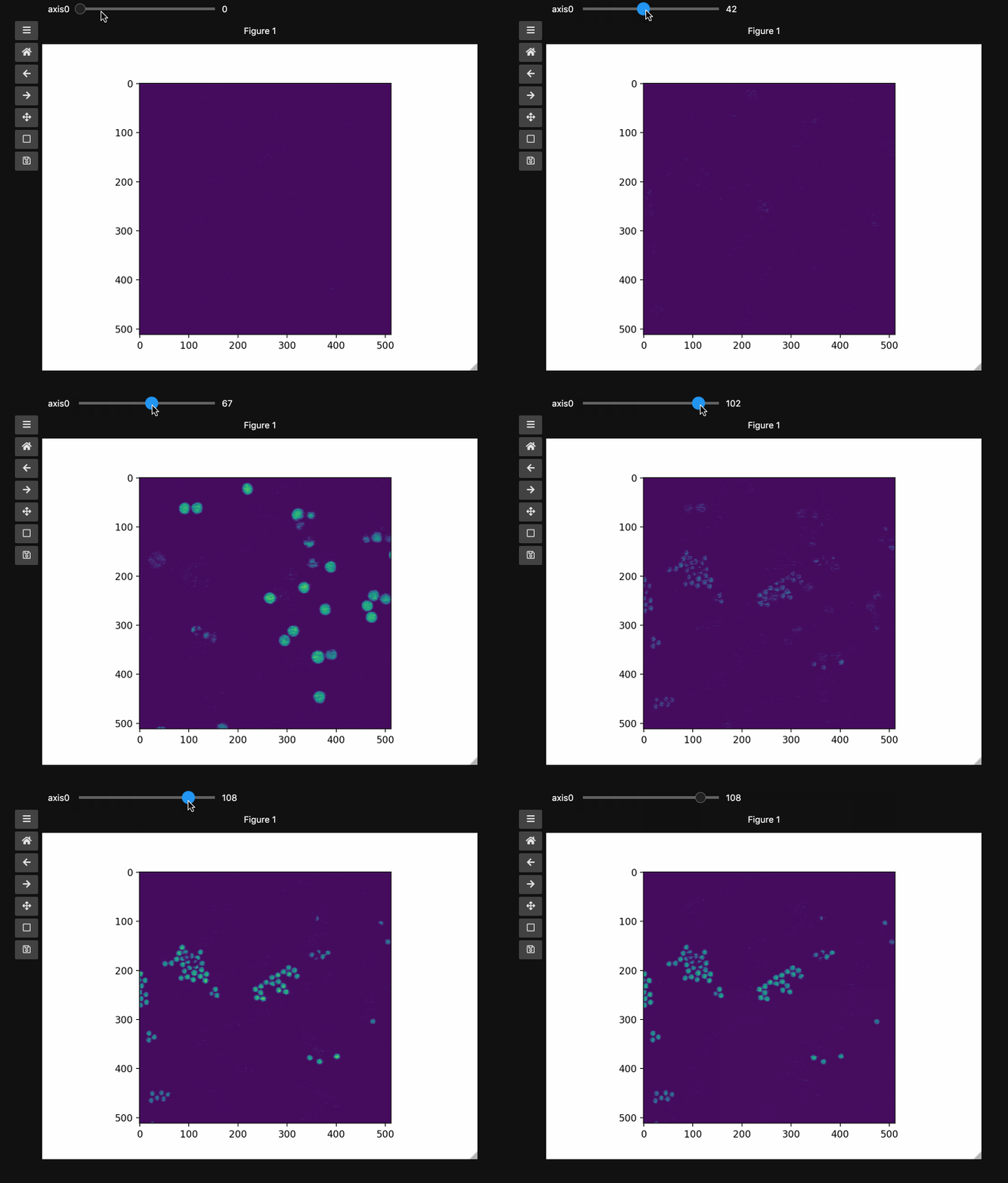
The hyperslicer() creates sliders to select slices of a multidimensional array (a hyperstack). It minimally requires an array whose last two (or three, if using RGB(A) images) dimensions are the image dimensions and all previous dimensions are taken to represent slices of the hyperstack. It will automatically generate sliders that select the the relevant slice along each dimension of the input array.
The example here uses a hyperspectral stimulated raman scattering stack of beads that are Raman active at different wavenumbers (No need to worry about the specifics but if you’re interested, the experimental setup is very similar to what is described here. You can download the dataset from here. The image contains two different bead species made of PMMA and polystyrene of different sizes. Some basic information for viewing and understanding the dataset is given in the table below.
Bead type |
Approx. Size |
Peak index |
Peak wavenumber |
|---|---|---|---|
PMMA |
10 µm |
66 |
2935 cm^(-1) |
Polystyrene |
5 µm |
111 |
3033 cm^(-1) |
import io

import matplotlib.pyplot as plt
import numpy as np
import requests

from mpl_interactions import hyperslicer

%matplotlib ipympl
# Get the dataset directly from github
response = requests.get("https://github.com/jrussell25/data-sharing/raw/master/srs_beads.npy")
response.raise_for_status()
beads = np.load(io.BytesIO(response.content))
print(beads.shape) # (126, 512, 512)
# Pass vmin and vmax for 8bit images otherwise the linear intensity slider appears useless
fig1, ax1 = plt.subplots()
control1 = hyperslicer(beads, vmin=0, vmax=255, play_buttons=True, play_button_pos="left")

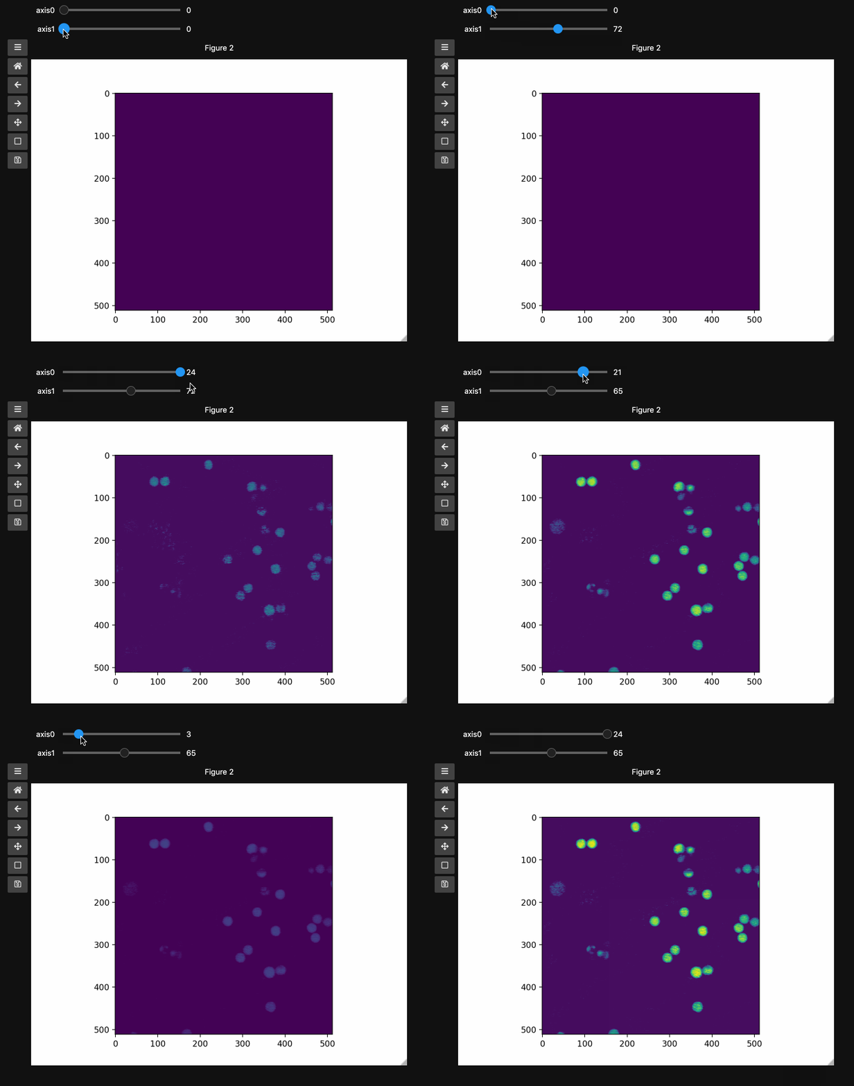
beads4d adds a linear scale from 0-1 over the intensities at each wavenumber and demonstrates the generalization to higher dimensional stacks.
beads4d = np.linspace(0, 1, 25)[:, None, None, None] * np.stack([beads for i in range(25)])
print(beads4d.shape) # (25, 126, 512, 512)
fig2, ax2 = plt.subplots()
controls2 = hyperslicer(beads4d, vmin=0, vmax=255)

Names and Values for sliders#
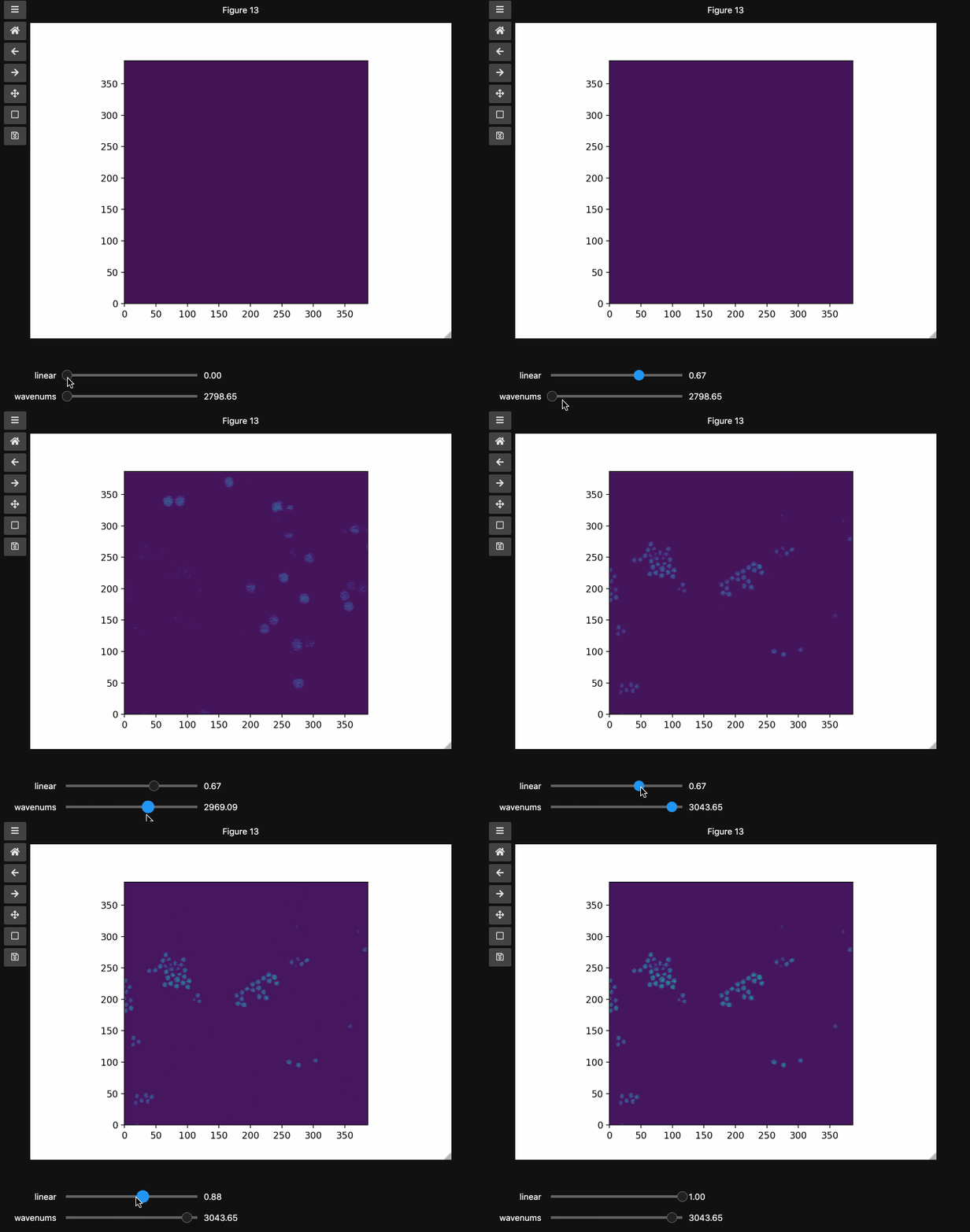
You can also provide names and or limits to map the sliders from the integers to other numbers. For instance in the beads4d dataset, we can replace the first dimension with the relative intensity of the image in [0,1] and the first dimension with the relevant spectrosocpic values, Raman wavenumbers.
The cells below show the two valid ways to generate these hyperslicers, first by passing a start, stop tuple and second by passing a full array containing the slider values. hyperslicer() handles mapping these values to indices to slice the data. Either of these options can be mixed with None or simply omitted to generate the default integer valued sliders as above. Separately, you can provide names for each axis to replace the axis0 style labels used by default.
Note: Matplotlib sliders currently do not support displaying different values than the slider actually uses internally. Thus for hyperslicer() matplotlib sliders must be IntSliders that display the values of the index of the array that you are accessing.
wns = np.linspace(2798.6521739130435, 3064.95652173913, beads4d.shape[1])
fig3, ax3 = plt.subplots()
controls3 = hyperslicer(
    beads4d, vmin=0, vmax=255, axis0=(0, 1), axis1=wns, names=("linear", "wavenums")
)

Instead of specifying the values for each axis and the names separately, one can use the axes keyword argument which expects a 2-tuple for each axis containing (name, (start, stop)) or (name, slider_value_array). Using the axes argument is probably the best way to use hyperslicer().
fig4, ax4 = plt.subplots()
controls4 = hyperslicer(beads4d, vmin=0, vmax=255, axes=(("linear", (0, 1)), ("wavenums", wns)))
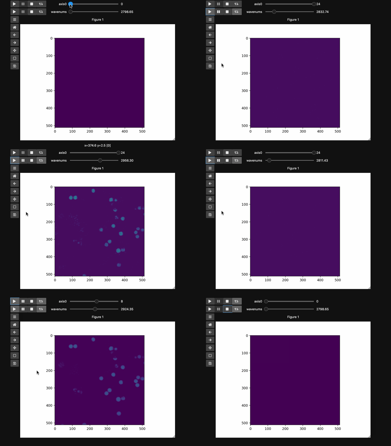
If you’re looking for ImageJ/FIJI type experience, adding play buttons is a nice touch.
fig5, ax5 = plt.subplots()
controls5 = hyperslicer(
    beads4d,
    vmin=0,
    vmax=255,
    axes=(("linear", (0, 1)), ("wavenums", wns)),
    play_buttons=True,
    play_button_pos="left",
)

Other ways of specifying axes#
All of the below are valid calls to hyperslicer, which generally supports omitting any of the labels or names while falling back to integer valued sliders. If you come across bugs relating to omitting values or passing None, please feel free to open an issue.
fig6, ax6 = plt.subplots()
controls6 = hyperslicer(beads4d, vmin=0, vmax=255, axes=(("linear", (0, 1)), "wavenums"))
fig7, ax7 = plt.subplots()
controls7 = hyperslicer(beads4d, vmin=0, vmax=255, axes=(("linear", 0, 1), "wavenums"))
fig8, ax8 = plt.subplots()
controls8 = hyperslicer(beads4d, vmin=0, vmax=255, axes=((0, 1), "wavenums"))
Hyperslicer with Xarray#
Xarray is a library for having named dimensions on an array and hyperslicer supports them natively. So if you’re going to go to the trouble of defining the axes argument you might think about just using xarray and doing it once per dataset and letting xarray keep track of them. Then hyperslicer will just access the information for you.
Xarray also integrates with dask for lazy data loading so if your data is large this is a good way to process them and now you can selectively visualize these lazy arrays with hyperslicer. Here we will just demonstrate the basics with an in memory xarray but the out of memory case is similar albeit slower to render.
import xarray as xr
# Define the coordinates for the xarray as a dict of name:array pairs
# Intensity is arbiratrily made to be 0-1
# Wns = Wns is relevant spectroscopic unit in cm^-1 as above
# X,Y = actual dimensions of the images in microns from microscope metadata
coords = {
    "linear": np.linspace(0, 1, beads4d.shape[0]),
    "wavenums": wns,
    "X": np.linspace(0, 386.44, 512),
    "Y": np.linspace(0, 386.44, 512),
}
x_beads4d = xr.DataArray(beads4d, dims=coords.keys(), coords=coords)
fig9, ax9 = plt.subplots()
controls9 = hyperslicer(x_beads4d, vmin=0, vmax=255)

Hyperslicer also supports bare dask arrays with the same logic as numpy arrays.

