Plot#
The interactive plot function is available either as mpl_interactions.pyplot.interactive_plot() or as mpl_interactions.ipyplot.plot. It will behave equivalently to the normal matplotlib matplotlib.pyplot.plot() function if you don’t pass it any non-plotting kwargs. If you do pass in non-plotting kwargs and one or both of x or y is a function then the kwargs will be converted into widgets to control the function.
%matplotlib ipympl
import ipywidgets as widgets
import matplotlib.pyplot as plt
import numpy as np

import mpl_interactions.ipyplot as iplt
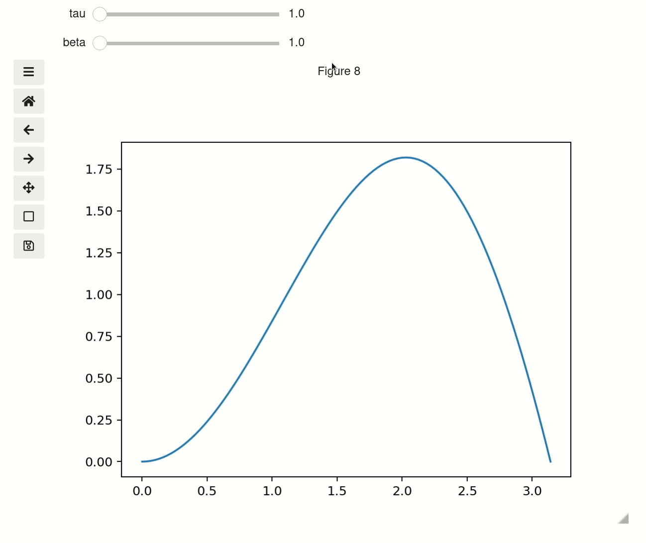
x = np.linspace(0, np.pi, 100)
tau = np.linspace(1, 10, 100)
beta = np.linspace(0.001, 1)


def f(x, tau, beta):
    return np.sin(x * tau) * x**beta


fig, ax = plt.subplots()
controls = iplt.plot(x, f, tau=tau, beta=beta)
Troubleshooting#
If instead of a plot you got an output that looks like this:
VBox([IntSlider(min=0, max=10 .....
and you are using jupyterlab then you probably need to install jupyterlab-manager:
conda install -c conda-forge nodejs=12
jupyter labextension install @jupyter-widgets/jupyterlab-manager
after the install and finishes refresh the browser page and it should work
set parameters with tuples#
When you use tuples with length of 2 or 3 as a parameter then it will be treated as an argument to linspace. So the below example is equivalent to first example
fig2, ax2 = plt.subplots()
controls2 = iplt.plot(x, f, tau=(1, 10, 100), beta=(1, 10))
Use sets for categorical values#
sets with three or fewer items will be rendered as checkboxs, while with more they will use the selection widget. Unfortunately sets are instrinsically disordered so if you use a set you cannot garuntee the order of the categoricals. To get around this if you have a set of single tuple it will be ordered. i.e. {('sin', 'cos')} will show up in the order: sin, cos. While {'sin', 'cos'} will show up in the order: cos, sin
def f(x, tau, beta, type_):
    if type_ == "sin":
        return np.sin(x * tau) * x**beta
    elif type_ == "cos":
        return np.cos(x * tau) * x**beta
    elif type_ == "beep":
        return x * beta / tau
    else:
        return x * beta * tau


fig3, ax3 = plt.subplots()
controls3 = iplt.plot(
    x, f, tau=(0.5, 10, 100), beta=(2, 10), type_={("sin", "cos", "beep", "boop")}
)
Using widgets for as parameters#
You can also pass an ipywidgets widget that has a value attribute
def f(x, tau, beta, type_):
    if type_ == "sin":
        return np.sin(x * tau) * x**beta
    elif type_ == "cos":
        return np.cos(x * tau) * x**beta


tau = widgets.FloatText(value=7, step=0.1)
fig4, ax4 = plt.subplots()
controls4 = iplt.plot(x, f, tau=tau, beta=(1, 10), type_={("sin", "cos")})
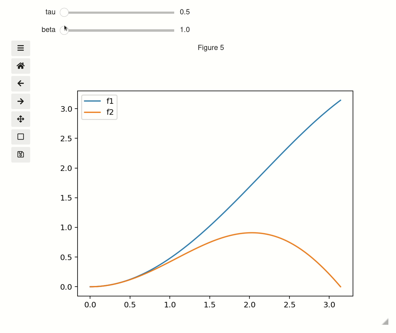
With multiple functions#
You have multiple interactive functions by passing the controls object to subsequent calls.
x = np.linspace(0, np.pi, 100)
tau = np.linspace(0.5, 10, 100)
beta = np.linspace(1, 10, 100)


def f1(x, tau, beta):
    return np.sin(x * tau) * x * beta


def f2(x, tau, beta):
    return np.sin(x * beta) * x * tau


fig, ax = plt.subplots()
controls = iplt.plot(x, f1, tau=tau, beta=beta, label="f1")
iplt.plot(x, f2, label="f2", controls=controls)
_ = plt.legend()
Or by using controls as a context manager. See Contextmanager for Controls object for complete examples of context manager usage.
fig, ax = plt.subplots()
controls = iplt.plot(x, f1, tau=tau, beta=beta, label="f1")
with controls:
    iplt.plot(x, f2, label="f2")
_ = plt.legend()
Styling of plot#
You can either use the figure and axis objects returned by the function, or if the figure is the current active figure the standard plt.__ commands should work as expected. You can also provide explicit plot_kwargs to the plt.plot() command that is used internally using the plot_kwargs argument
You can control how xlim/ylims behave using the x_scale/y_scale arguments. The options are:
stretch– never shrink the x/y axis but will expand it to fit larger valuesauto– autoscale the x/y axis for every plot updatefixed– always used the initial values of the limitsa
tuple– You can pass a value such as[-4,5]to have the limits not be updated by moving the sliders.
x_ = np.linspace(0, np.pi, 100)
tau = np.linspace(1, 10, 100)


def f_x(tau):
    return x_


def f_y(x, tau):
    return np.sin(x * tau) * x


fig, ax = plt.subplots()
controls = iplt.plot(
    f_x,
    f_y,
    tau=tau,
    xlim="stretch",
    ylim="auto",
    label="interactive!",
)

iplt.title("the value of tau is: {tau:.2f}", controls=controls["tau"])
# you can still use plt commands if this is the active figure
plt.ylabel("yikes a ylabel!")

# you can new lines - though they won't be updated interactively.
plt.plot(x, np.sin(x), label="Added after, not interactive")

_ = plt.legend()  # _ to capture the annoying output that would otherwise appear
Slider precision#
You can change the precision of individual slider displays by passing slider_format_string as a dictionary. In the below cell we give tau 99 decimal points of precision and use scientific notation to display it. The other sliders will use the default 1 decimal point of precision.
x = np.linspace(0, np.pi, 100)
tau = np.linspace(0.5, 10, 100)
beta = np.linspace(1, 10, 100)


def f1(x, tau, beta):
    return np.sin(x * tau) * x * beta


def f2(x, tau, beta):
    return np.sin(x * beta) * x * tau


fig, ax = plt.subplots()
controls = iplt.plot(x, f1, tau=tau, beta=beta, slider_formats={"tau": "{:.50e}"})
fixed y-scale#
You can also set yscale to anything the matplotlib will accept as a ylim
x = np.linspace(0, np.pi, 100)
tau = np.linspace(1, 10, 100)


def f(x, tau):
    return np.sin(x * tau) * x**tau


fig, ax = plt.subplots()
iplt.plot(x, f, tau=tau, ylim=[-3, 4], label="interactive!")

# you can still use plt commands if this is the active figure
plt.ylabel("yikes a ylabel!")
plt.title("Fixed ylim")

# you can new lines - though they won't be updated interactively.
plt.plot(x, np.sin(x), label="Added after, not interactive")

_ = plt.legend()  # _ to capture the annoying output that would otherwise appear